Deduplication Part 1: Rabin Karp for Variable Chunking
This is first post in a series of blog posts where we will discuss deduplication in a distributed data system. Here we will discuss different types of deduplication and various approaches taken in a distributed data systems to get optimum performance and storage efficiency.
But first basics of deduplication!![]()
“Data deduplication (often called “intelligent compression” or “single-instance storage”) is a method of reducing storage needs by eliminating redundant data. Only one unique instance of the data is actually retained on storage media, such as disk or tape” definition by searchstorage.techtarget.com
Deduplication goes good when we can break the data stream into smaller pieces called “Chunks”.
The process of breaking the data stream into chunks is called “chucking”.
Static or Fixed Block Chunking
The most naive and easiest way of chunking is breaking the data stream into fixed length-ed chunks say for example 256 bytes per chunk.
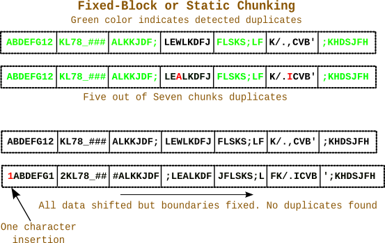
But the problem with this way of chunking is its not immune to the data displacement/shifting issue when an insert happens i.e when there is new data inserted in already chunked data stream there will be displacement/shifting of data.
This happens because the chunk boundaries are fixed, thus changing the content of every chunk after the insert as shown in the diagram. Thus all the data chunks after the insert change and thus considered new, even though they are deduplicates.
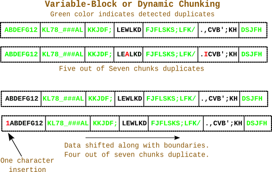
Variable or Dynamic chunking
The solution to this problem is chunking based on the content of the data stream. Well to do this we would require a way to identify a pattern on which we can chunk. The chunk boundaries will be guarded by pattern. This will have an implication on chunk size, i.e the chunk size will be variable in nature. And hence its called “Variable Chunking”. As you can see this scheme of chunking is immune from the data displacement/shifting issue because the chunk boundaries are guarded by pattern.
To find the chunking pattern we have to use a [rolling hash]. The idea is to define a data window on the data stream, which has finite and predefined size of say “N”. Now using a hashing technique calculate a hash on the window. Check if the hash matches a predefined “finger_print”.
- If the “finger_print” does match the calculated rolling hash on the window, mark the Nth element as the chuck boundary.
- If the “finger_print” doesn’t match the calculated rolling hash on the window, slide the window by one element and recalculate the rolling hash. Repeat this until you find a match.
To search for the chunk pattern the Rabin-Karp Rolling Hash is used. If n is the window size then for a window from i to i + (N-1) the hash would be calculated using the following polynomial
H (i, i+n-1) = (P^(n-1))*a[i] + (P^(n-2))*a[i+1] +...+P a[i+n] + a[i+n-1]
where a[] is a data window of size n , starting from i to i+n-1,
P is a prime number (for better hash results).
The challenge to use this polynomial in a computer system is the value of the hash will overflow even an 64bit unsigned integer.Therefore to solve this we use a modulo
m on H i.e H%m and call it hash and then compare it with the finger_print
Now to calculate the **hash** we take the help of [modulo arithmetic]
  ( a * b ) %m = ( (a % m ) * b ) % m = ( (a % m ) * (b % m) ) % m
  ( a + b ) %m = ( (a % m ) + b ) % m = ( (a % m ) + (b % m) ) % m
So that we can calculate the **hash** by building a [recurrence relation].
Now when n=1 i,e the window size is 1,
H(n=1) = ( P^0 ) * a[i] = a[i]
and
hash(n=1) = H(n=1) %m = a[i] % m --------------> (1)
when n=2 i,e the window size is 2,
H(n=2) = ( P^1 ) * a[i] + a[i+1] = P*a[i] + a[i+1]
and
hash(n=2) = H(n=2) %m = {  P*a[i] + a[i+1]  } % m --------------> (2)
                      = { P * ( a[i]%m ) + a[i+1] } % m //using modulo arithmetic
                      = { P * hash(n=1) + a[i+1] } % m // from (1)
when n=3 i,e the window size is 3,
H(n=3) = (P^2)*a[i] + P*a[i+1] + a[i+2]
and
hash(n=3) = H(n=3) %m = { (P^2)*a[i] + P*a[i+1] + a[i+2]  } % m
                      = { P * { ( P*a[i] + a[i+1] ) %m } + a[i+2] } % m //using modulo arithmetic
                      = { P * hash(n=2) + a[i+2] } % m //  from (2)
As we can see we can have a [recurrence relation] between hash(n=k) and hash(n=k-1)
hash(n=k) = { P * hash(n=k-1) + a[k-1] }
Similarly we can have a [recurrence relation] between (P^k) % m and (P ^ {k-1}) %m.
Lets POWER(n=k) = (P^k)%m
POWER(n=k) = (P^k) %m = ( (P^ {k-1} ) * P ) % m
i.e
POWER(n=k) = ( POWER(n={k-1}) * P ) % m
The above will be used later, just note it for now.
Using the above recurrence relation for hash(n=k) we can calculate the first chunking window hash
To have high performing chunking algorithm we cannot repeat the above for every subsequent window. We can to use the previous chunking windows hash and calculate the next chucking windows hash, as the only change during a window slide is of 2 elements i.e an outgoing element a[i] and an incoming element a[1+n]
Let have a re-look at out polynomial
H (i, i+n-1) = (P^(n-1))*a[i] + (P^(n-2))*a[i+1] + ...+P a[i+n] + a[i+n-1]
For the subsequent window the polynomial would be
H (i+1, i+n) = (P^(N-1))*a[i+1] + (P^(N-2))*a[i+2] +...+P*a[i+n-1] + a[i+n] --------------- (3)
Multiply H((i, i+n-1)) by P
H (i, i+n-1) * P = ( (P^(n-1))*a[i] + (P^(n-2))*a[i+1] +...+P a[i+n] + a[i+n-1] ) * P
                = (P^(n))*a[i] + (P^(n-1))*a[i+1] +...+ (P^2 )a[i+n] + P*a[i+n-1]


Subtract (P^n)*a[i] & Adding  a[i+n] on both the sides of the equation
                                = H (i+1, i+n) // from (3)


H (i, i+n-1) * P - (P^N)*a[i] + a[i+n] =  { (P^(n-1))*a[i+1] +...+ (P^2 )a[i+n] + P*a[i+n-1] } + a[i+n]
i,e
H (i+1, i+n)  = H (i, i+n-1) * P - (P^n)*a[i] + a[i+n]
Applying % m on the above equation
H (i+1, i+n) % m = { H (i, i+n-1) * P - (P^n)*a[i] + a[i+n] } % m
i.e
hash(i+1, i+n) = { H (i, i+n-1) * P - (P^n)*a[i] + a[i+n] } % m
               = { (H (i, i+n-1)%m) * P - (P^n % m)*a[i] + a[i+n] } % m //using modulo arithmetic
Therefore,
hash(i+1, i+n) = = { hash(i,i+n-1) * P - POWER(n)*a[i] + a[i+n] } % m ------------ (4)
Now using (4) we have a recurrence relation using which we can calculate the hash of the next chunk window using previous chunk window hash ( hash(i,i+n-1)), outgoing element (a[i]) and incoming element (a[i+n]) i.e
hash(next) = = { hash(prev) * P – POWER(n)outgoing + incoming } % m
Reference:
- https://moinakg.wordpress.com/tag/rabin-fingerprint/
- https://en.wikipedia.org/wiki/Rolling_hash
- http://en.wikipedia.org/wiki/Rabin%E2%80%93Karp_algorithm
- http://en.wikipedia.org/wiki/Recurrence_relation
- https://www.hackerearth.com/notes/modular-arithmetic/
- http://infolab.stanford.edu/~ullman/mmds/book.pdf
Related work:
- https://github.com/YADL/yadl
- https://gluster.readthedocs.org/en/latest/presentations/Dedupe_nmamit.odp

![]()